J.P.M Quantitative Project

J.P.M Quantitative

🔥Task1

选取五只股票进行有效前沿的绘制以及给定预期收益的最佳持仓配比求解

🍴 具体任务实现的算法

1.有效前沿的绘制：sco

2.最佳持仓配比求解：cvxopt/sco

The efficient frontier represents the best combinations of risk and expected return, which offer the highest expected return at a given level of risk or the lowest risk for a given expected return.
有效前沿作为代表了一组风险和预期回报之间的最佳组合，这些组合在给定的风险水平下提供了最高的预期回报，或者在给定的预期回报下具有最低的风险。

基础数据及其特征展示

```
    pip install cvxopt
    pip install yfinance #下载股票数据

```
    import numpy as np
    import pandas as pd  
    import matplotlib.pyplot as plt  
    from cvxopt import matrix, solvers
    import yfinance as yf 

    # 获取股票数据  
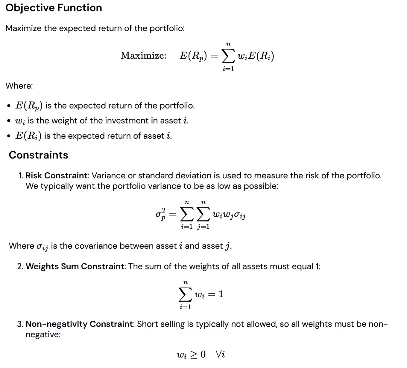
    tickers = ['GOOG', 'MSFT', 'AAPL', 'NVDA', 'AMZN']  
    data = yf.download(tickers, start='2024-01-01', end='2024-10-01')['Adj Close']

    data.shift(1) #创造一行空行用于计算收益率

    #将股票按照初始交易日进行归一化处理并可视化
    (data/data.iloc[0]).plot(figsize=(10,6),grid=True)

算法实现

投资组合可行解

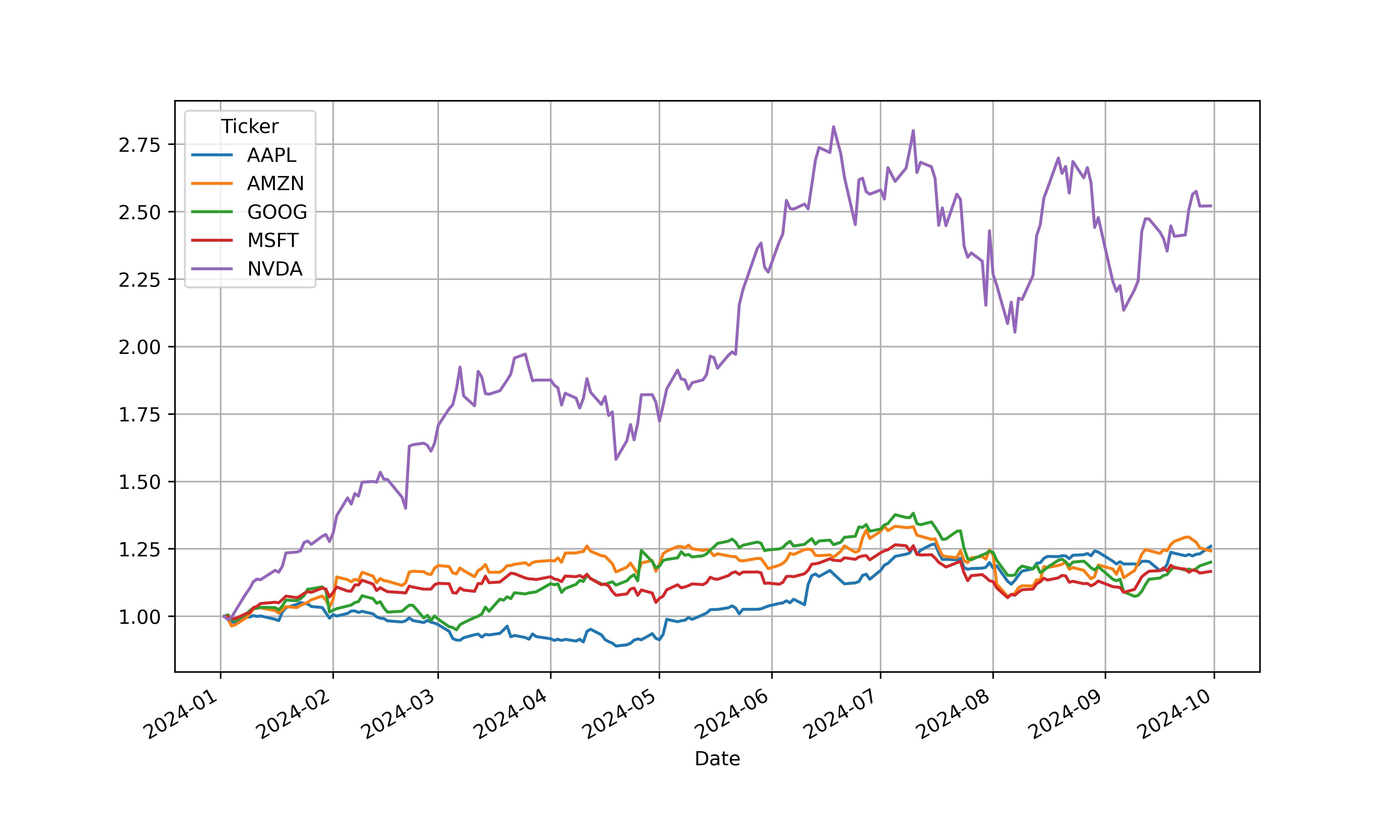
```
    #随机进行2000次模拟  
    #Rp_list,Vp_list分别存储每个模拟投资的预期收益率和波动率
    n=5   #五只股票五个投资组合
    I=2000
    Rp_list=np.ones(I)  #预期收益率
    Vp_list=np.ones(I)  #波动率
    SR_list=np.ones(I)  #夏普比率

    #模拟过程
    for i in np.arange(I):
       x=np.random.rand(n)  #生成n个随机权重
       weights=x/sum(x)     #权重归一化，使其和为1
       Rp_list[i]=np.sum(weights*Manual_LR)  
       Vp_list[i]=np.sqrt(np.dot(weights,np.dot
(Cov_LR,weights.T)))  
       SR_list[i]=Rp_list[i]/Vp_list[i]

    #展示结果    
    plt.figure(figsize=(8, 4), dpi=100, facecolor='white')  
    plt.scatter(Vp_list, Rp_list)  
    plt.title('The relationship between expected portfolio return and volatility', pad=20)  
    plt.xlabel('Volatility', labelpad=20)  
    plt.ylabel('Expected Return', labelpad=20)  
    plt.grid()

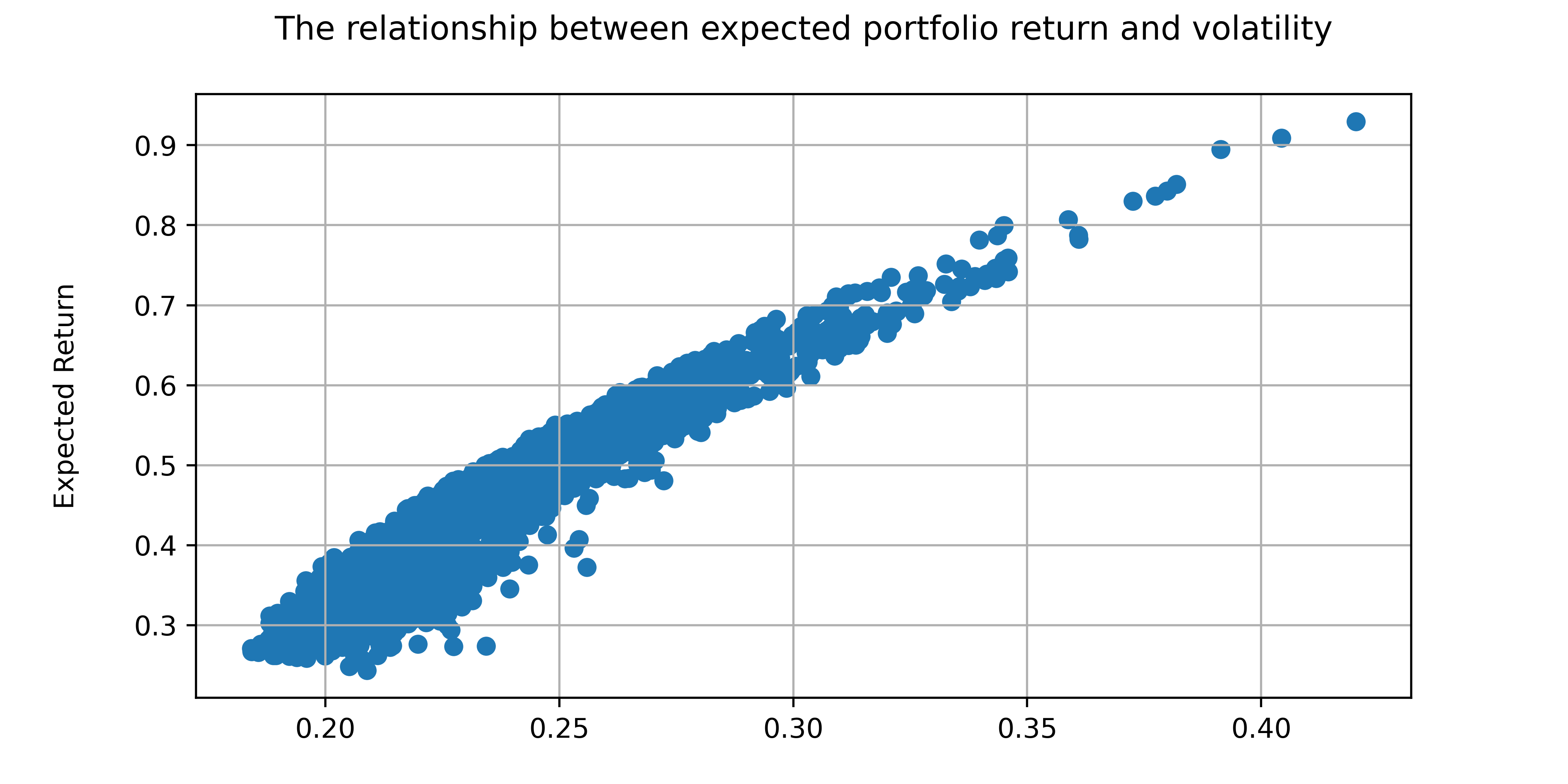
投资组合的有效前沿

```
    import scipy.optimize as sco

   #必要参数构建
    def f(w):
       w=np.array(w)
       Rp_opt=np.sum(w*Manual_LR)
       Vp_opt=np.sqrt(np.dot(w,np.dot(Cov_LR,w.T)))
       return np.array([Rp_opt,Vp_opt])

    def Vmin_f(w):
       return f(w)[1]

    cons=({'type':'eq','fun':lambda x:np.sum(x)-1},{'type':'eq','fun':lambda x:f(x)[0]-0.15})
    bnds=((0,1),(0,1),(0,1),(0,1),(0,1))

    #权重决定重要性
    w0=np.array([0.2, 0.2, 0.2, 0.2, 0.2])  
    result=sco.minimize(fun=Vmin_f,x0=w0,method='SLSQP',bounds=bnds,
    constraints=cons)
    cons_vmin=({'type':'eq','fun':lambda x:np.sum(x)-1})
    result_vmin=sco.minimize(fun=Vmin_f,x0=w0,
    method='SLSQP',bounds=bnds,constraints=cons_vmin)

    Vp_vmin=result_vmin['fun']
    Rp_vmin=np.sum(Manual_LR*result_vmin['x'])
 
    Rp_target=np.linspace(Rp_vmin,0.95,300)
    Vp_target=[]

    for r in Rp_target:
      cons_new=({'type':'eq','fun':lambda x:np.sum(x)-1},{'type':'eq','fun':lambda x:f(x)[0]-r})
      result_new=sco.minimize(fun=Vmin_f,x0=w0,
      method='SLSQP',bounds=bnds,constraints=cons_new)
       Vp_target.append(result_new['fun'])

    #展示结果    
     plt.figure(figsize=(8, 4))  
     plt.scatter(Vp_list,Rp_list,c=SR_list, cmap='YlGnBu', marker='o')  
     plt.colorbar(label='Sharpe Ratio')  
     plt.plot(Vp_target,Rp_target,'r-',label="efficient frontier")
     plt.scatter(sdp, rp, marker='*', color='r', s=300, label='Max Sharpe Ratio')  
     plt.title('Efficient Frontier')  
     plt.xlabel('Annualized Volatility')  
     plt.ylabel('Annualized Return')  
     plt.legend(labelspacing=0.8)  
     plt.show()

必要参数设置

The price-to-earnings ratio cannot symmetrically account for both increases and decreases in stock prices; the effects of a 50% increase and a 50% decrease do not offset each other. Calculating multi-period returns is prone to cumulative errors, making it suitable for analyzing discontinuous income events such as dividends and other one-time gains.
Logarithmic Return: Assuming the market operates under continuous compounding, logarithmic returns more accurately reflect true gains. They exhibit symmetrical fluctuations and allow multi-period returns to be simply summed without cumulative error. This approach better aligns with the assumption of normal distribution. Logarithmic returns are particularly suitable for long-term investments and complex financial models.

股价收益率不能处理对称处理上涨和下跌，增加50%和减少50%的影响不会相互抵消,多期收益计算容易产生累积误差，适合分析不连续性的收益事件，如分红和其他一次性收益。
对数收益率：假设市场是连续复利的，对数收益率更反映真实收益，上下波动对称，且多期收益可以简单相加而不产生累积误差，更适合正态分布假设,长期投资和复杂的金融模型适合使用对数收益率。

```
    #计算股票的对数收益率并且展示描述性统计指标
    Log_return=np.log(data/data.shift(1))
    #计算股票的年平均收益率  通过计算该序列的算术平均值的到平均对数收益率
    Manual_LR=Log_return.mean()*252
    #计算股票收益率的年化波动率  计算平均波动率后年化
    Vol_LR=Log_return.std()*np.sqrt(252)
    #计算股票的协方差矩阵并进行年化处理
    Cov_LR=Log_return.cov()*252
    #计算股票的相关系数矩阵
    Corr_LR=Log_return.corr()

资本市场线

``` 
    Rf=0.03  #无风险利率
    def F(w):
       w=np.array(w)
       Rp_opt=np.sum(w*Manual_LR)
       Vp_opt=np.sqrt(np.dot(w,np.dot(Cov_LR,w.T)))
       Slope=(Rp_opt-Rf)/Vp_opt
       return np.array([Rp_opt,Vp_opt,Slope])

    def Slope_F(w):
          return -F(w)[-1]

    w1=np.array([0.2, 0.2, 0.2, 0.2, 0.2])
    cons_Slope=({'type':'eq','fun':lambda x:np.sum(x)-1})
    result_slope=sco.minimize(fun=Slope_F,x0=w1,method='SLSQP',bounds=bnds,
constraints=cons_Slope)

    Rm=np.sum(Manual_LR*wm)
    Vm=(Rm-Rf)/Slope
    Rp_CML=np.linspace(Rf,0.95,200)
    Vp_CML=(Rp_CML-Rf)/Slope

    #展示结果    
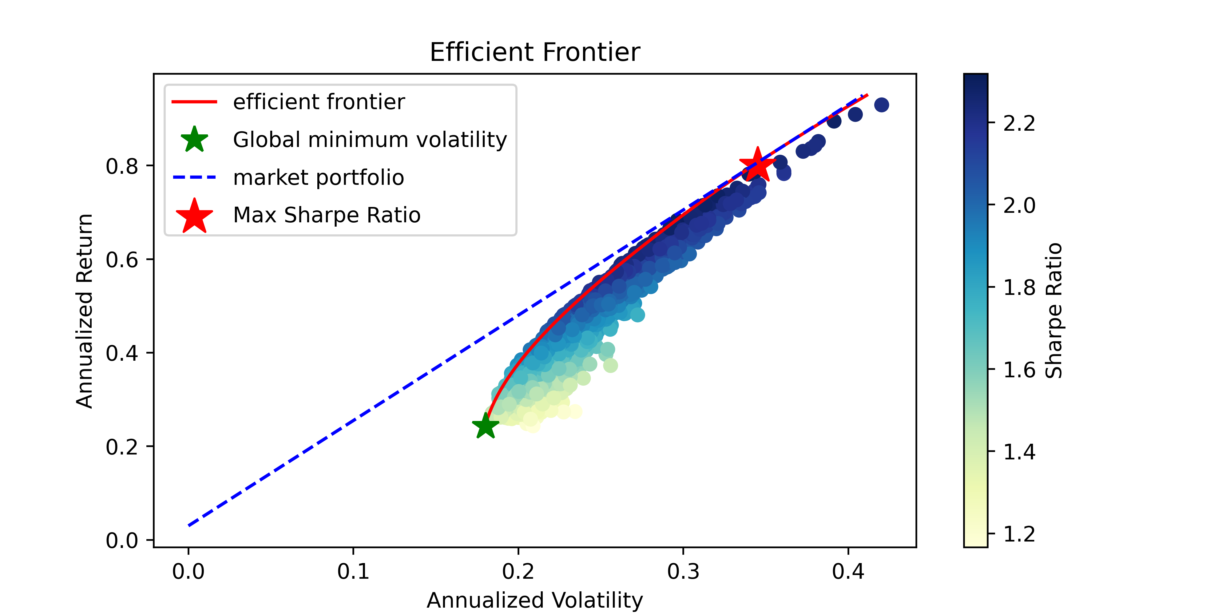
    plt.figure(figsize=(8, 4))  
    plt.scatter(Vp_list,Rp_list,c=SR_list, cmap='YlGnBu', marker='o')  
    plt.colorbar(label='Sharpe Ratio')  
    plt.plot(Vp_target,Rp_target,'r-',label="efficient frontier")
    plt.plot(Vp_vmin,Rp_vmin,'g*',label='Global minimum volatility',markersize=13)
    plt.plot(Vp_CML,Rp_CML,'b--',label='market portfolio',markersize=13)
    plt.scatter(sdp, rp, marker='*', color='r', s=300, label='Max Sharpe Ratio')  
    plt.title('Efficient Frontier')  
    plt.xlabel('Annualized Volatility')  
    plt.ylabel('Annualized Return')  
    plt.legend(labelspacing=0.8)  
    plt.show()

基于cvxopt的资产组合配置

```
   #计算每个股票日收益率的百分比变化并且移除掉有缺失值的行  
   returns = data.pct_change().dropna()  
 
   cov_matrix = returns.cov() * 252  # 年化协方差矩阵  
   print(cov_matrix)  

   #选用cvxopt，作为凸优化问题的工具的默认参数已经比较高效，如果想进一步优化性能，可以
   #通过优化矩阵表示（如利用系数矩阵）和调节求解器参数（如迭代次数、容忍度）来改善性能

   #投资组合优化  
   def optimize_portfolio(cov_matrix, mean_returns, target_return):  
       n = len(mean_returns)  
       P = matrix(cov_matrix.values)  
       q = matrix(np.zeros((n, 1)))  
       G = matrix(np.vstack((-np.array(mean_returns), -np.identity(n))))  
       h = matrix(np.hstack((-target_return, np.zeros(n))))  
       A = matrix(1.0, (1, n))  
       b = matrix(1.0)  

       solvers.options['show_progress'] = False  
       sol = solvers.qp(P, q, G, h, A, b)  

       return sol['x']  

   # 目标返回  
   target_return = 0.1  # 10% 的目标年化收益率  
   mean_returns = returns.mean() * 252  

   optimal_weights = optimize_portfolio(cov_matrix, mean_returns, target_return)  
   print("\nOptimal Portfolio Weights:")  
   print([round(w, 4) for w in optimal_weights])  

🔥Task2

基于Black-Litterman的最佳持仓配比求解

Background

①The Markowitz model typically accepts inputs derived either from historical data or from scenario analysis. Scenario analysis suffers from excessive subjectivity and arbitrariness; therefore, the historical-data approach—feeding the model with asset return means and covariances—is more common in practice. However, this approach has notable drawbacks: the future distribution of asset returns need not match the historical distribution, and historical extrapolation is vulnerable to structural instability (e.g., time-varying means, volatilities, and correlations). Moreover, Markowitz allocations are highly sensitive to input parameters; even small errors in estimated means or covariances can induce large swings in portfolio weights, undermining implementability and robustness.
②The Black–Litterman model was developed precisely to address these issues. Its central idea is to combine the investor’s subjective views on broad asset classes with the market’s equilibrium returns (the prior expected returns) via a Bayesian updating scheme, thereby producing calibrated posterior expected returns. In this formulation, the prior distribution of expected returns can be modeled as a multivariate normal prior in the Bayesian sense; the investor’s subjective views act as the likelihood function (i.e., new information reflecting judgments formed from external signals about asset return dynamics); and the posterior expected returns are obtained from the posterior distribution.
③In essence, the model fuses investor views with equilibrium returns to generate a new vector of expected returns. The prior is modeled as a multivariate normal distribution, the investor views constitute the likelihood, and the posterior expected returns are derived from the posterior distribution.

①Markowitz模型输入参数包括历史数据法和情景分析法两种方法,情景分析法的缺点是主观因素,随意性太强,因此使用历史数据法, 将资产的均值和协方差输入模型是比较常见的作法. 此做法存在显著不足:未来的资产收益率分布未必与历史分布一致，同时历史外推存在结构性不稳定风险（如均值、波动率、相关性随时间漂移）。此外, Markowitz 模型结果对输入参数高度敏感，微小的均值或协方差误差可能导致配置权重发生巨幅变化，进而影响可实施性与稳健性。
②Black-Litterman模型就是基于此的改进. 其核心思想是将投资者对大类资产的主观观点与市场均衡收益率（先验预期收益）进行贝叶斯式融合，形成经过校准的新的预期收益（后验预期收益. 这里的先验预期收益率的分布可以是贝叶斯推断中的先验概率密度函数的多元正态分布形式,投资者的主观观点就是贝叶斯推断中的似然函数(可以看作新的信息, 因为做出主观判断必然是从外界获取得到了这些资产的收益率变化信息), 而相应的, 后验预期收益率也可以从后验概率密度函数中得到
③核心思想是将投资者对大类资产的观点与市场均衡收益率相结合,从而形成新的预期收益率，是贝叶斯推断中的先验概率密度函数的多元正态分布形式,投资者的主观观点是似然函数, 后验预期收益率从后验概率密度函数中得到。

求解步骤

①Prior construction:The covariance matrix used in the prior density is typically based on the covariance matrix of historical returns.
Determine the vector of market-expected returns, i.e., the prior mean of expected returns. Alternatively, one may infer the market-implied equilibrium return vector from existing expected returns and variances (reverse optimization). When using this approach, the risk-free rate must be specified.
②Incorporation of investor views:Integrate investor views by specifying the views’ mean vector (reflecting the investor’s directional/relative expectations), and the views’ uncertainty via a views covariance (often linked to the variance of the view variables and the investor’s confidence).
③Notation and calibration parameters:
τ: a scalar that scales the covariance of the equilibrium returns, often interpreted as an adjustment reflecting confidence in the prior (smaller τ indicates higher confidence in the prior).
Σ: the covariance matrix of historical asset returns.
P: the pick matrix mapping assets to views (the “views matrix”).
Ω: the covariance matrix associated with the likelihood (the uncertainty of investor views). A common specification is a diagonal matrix with entries derived from the diagonal of the P^T(τΣ)P.
Π:the prior (equilibrium) expected returns.
④Portfolio optimization:Feed the posterior (adjusted) expected returns and the chosen covariance matrix back into the Markowitz mean–variance optimizer to obtain the final portfolio weights.

①通常使用历史数据估计预期收益率的协方差矩阵作为先验概率密度函数的协方差的基础.
确定市场预期之收益率向量, 也就是先验预期收益之期望值. 作为先验概率密度函数的均值. 或者使用现有的期望值和方差来反推市场隐含的均衡收益率(Implied Equilibrium Return Vector), 不过在使用这种方法时, 需要知道无风险收益率Rf的大小.
②融合投资人的个人观点,即根据历史数据(看法变量的方差)和个人看法(看法向量的均值)
③τ是均衡收益率协方差的调整系数,可以根据信心水平来判断.τ是均衡收益率协方差的调整系数， Sigma是历史资产收益率的协方差矩阵, P是投资者的观点矩阵,Ω 是似然函数(即投资者观点函数)中的协方差矩阵,其值为P^T(τΣ)P的对角阵, Π是先验收益率的期望值
④投资组合优化：将修正后的期望值与协方差重新代入马科维茨投资组合模型求解

🍴 具体任务实现的算法

```
# Black-Litterman 模型定义  
# tau 是一个标量参数，
#通常取值在 0 到 1 之间。它表示我们对市场均衡的信心相对于样本信息的程度。
# tau通常选 1/选观察的交易日长度
def blacklitterman(returns, tau, P, Q):  
    mu = returns.mean()  
    sigma = returns.cov()  
    pil = np.expand_dims(mu, axis=0).T  # 市场均衡预期收益率（Π）  
    ts = tau * sigma  
    ts_inv = linalg.inv(ts)  
    Omega = np.dot(np.dot(P, ts), P.T) * np.eye(Q.shape[0])  # 观点评价矩阵  
    Omega_inv = linalg.inv(Omega)  
    # 计算后验预期收益率  
    er = linalg.inv(ts_inv + np.dot(np.dot(P.T, Omega_inv), P)) @ (np.dot(ts_inv, pil) + np.dot(np.dot(P.T, Omega_inv), Q))  
    # 计算后验协方差矩阵  
    posteriorSigma = linalg.inv(ts_inv + np.dot(np.dot(P.T, Omega_inv), P))  
    return [er, posteriorSigma]  
```

````python
```

# 定义投资者的观点  
pick1 = np.array([1, 0, 1, 1, 1])  # 观点1涉及GOOG, AAPL, NVDA, AMZN  
q1 = np.array([0.003 * 4])        # 对应的观点预期收益率  

pick2 = np.array([0.5, 0.5, 0, 0, -1])  # 观点2是GOOG和MSFT的组合比AMZN表现更好  
q2 = np.array([0.001])                  # 对应的观点预期收益率  

P = np.array([pick1, pick2])  
Q = np.array([q1, q2])

# 计算 Black-Litterman 后验预期收益率和协方差矩阵  
res = blacklitterman(log_return, 1/252, P, Q)  

# res[0]: 后验均值   # res[1]：后验协方差矩阵  

```

#最小方差组合的资产配置权重 (blminVar)
# 定义最小方差组合计算函数  
def blminVar(cov_matrix):  
    n = cov_matrix.shape[0]  
    ones = np.ones(n)  
    inv_cov = linalg.inv(cov_matrix)  
    weights = inv_cov @ ones / (ones.T @ inv_cov @ ones)  
    return weights  

# 计算最小方差组合的权重  
weights = blminVar(res[1])  

# 将结果转换为 pandas Series，方便展示  
weights_series = pd.Series(weights, index=tickers) 

```

# 可视化权重分布  
plt.figure(figsize=(10,6))  
weights_series.plot(kind='bar')  
plt.title('Minimum Variance Portfolio Weights (Black-Litterman)')  
plt.ylabel('Weight')  
plt.xlabel('Assets')  
plt.grid(True)  
plt.savefig('Minimum Variance Portfolio Weights (Black-Litterman).png', dpi=500)
plt.show()

```

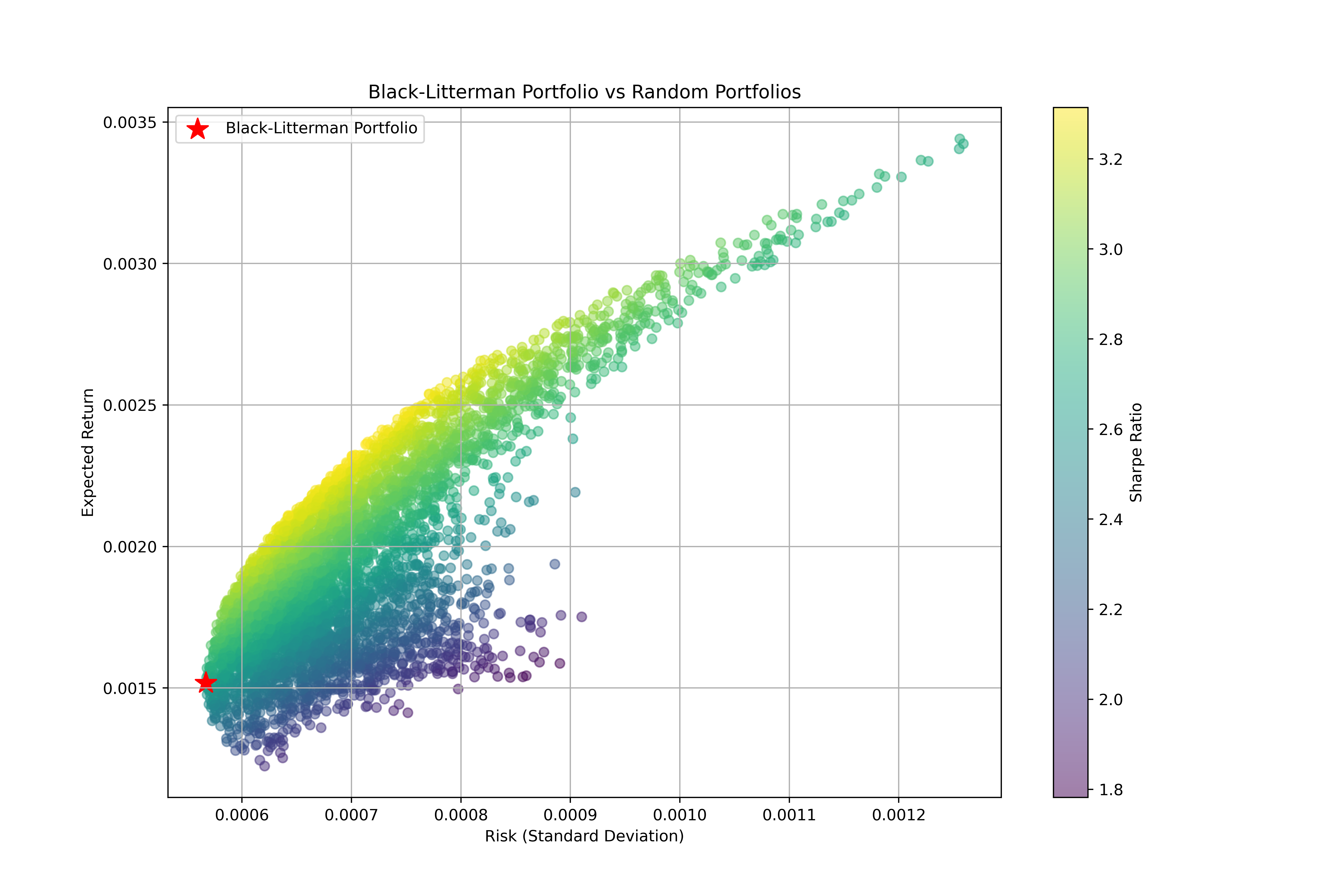
#2. 比较 Black-Litterman 组合与随机组合的预期收益和风险  

weights_BL=weights_series
# 计算 Black-Litterman 组合的预期收益和风险  
mu_BL = res[0].flatten()  
portfolio_return_BL = np.dot(weights_BL, mu_BL)  
portfolio_variance_BL = np.dot(weights_BL, np.dot(res[1], weights_BL))  
portfolio_std_BL = np.sqrt(portfolio_variance_BL)  

# 生成随机组合  
num_portfolios = 5000  
np.random.seed(42)  # 为了结果可重复  

random_weights = np.random.dirichlet(np.ones(len(tickers)), size=num_portfolios)  
random_returns = random_weights @ mu_BL  
random_variances = np.einsum('ij,ik,jk->i', random_weights, random_weights, res[1])  
random_std = np.sqrt(random_variances)  

# 计算随机组合的预期收益和风险  
random_returns = random_weights @ mu_BL  
random_std = np.sqrt(random_variances)  

# 计算随机组合的夏普比率（假设无风险利率为0）  
sharpe_random = random_returns / random_std  
sharpe_BL = portfolio_return_BL / portfolio_std_BL  

# 3. 可视化比较  

plt.figure(figsize=(12,8))  
plt.scatter(random_std, random_returns, c=sharpe_random, cmap='viridis', alpha=0.5)  
plt.colorbar(label='Sharpe Ratio')  
# 绘制 Black-Litterman 组合  
plt.scatter(portfolio_std_BL, portfolio_return_BL, color='red', marker='*', s=200, label='Black-Litterman Portfolio')  
plt.title('Black-Litterman Portfolio vs Random Portfolios')  
plt.xlabel('Risk (Standard Deviation)')  
plt.ylabel('Expected Return')  
plt.legend()  
plt.grid(True)  
plt.savefig('BL_Portfolio.png', dpi=500)
plt.show()  

```

# 初始化一个DataFrame来存储所有随机组合的累计收益率  
num_simulations =10000  
np.random.seed(42)  # 为了可重复性  

# 计算简单收益率并去除缺失值  
simple_return = data.pct_change()  # 计算简单收益率  
simple_return = simple_return.dropna(how='all')  # 去除缺失值


# 初始化一个DataFrame来存储所有随机组合的累计收益率  
cumulative_random_all = pd.DataFrame(index=simple_return.index)  
final_random_returns = []  
def calculate_cumulative_returns(simple_return, weights):  
    """  
    计算组合的累计收益率。  

    参数:  
    - simple_return: DataFrame，每个资产的简单收益率。  
    - weights: 数组或列表，资产的权重。  

    返回:  
    - cumulative_returns: Series，组合的累计收益率。  
    """  
    # 计算组合的加权收益率  
    portfolio_return = (simple_return @ weights)  
    
    # 计算累计收益率  
    cumulative_returns = (1 + portfolio_return).cumprod() - 1  
    
    return cumulative_returns

# 计算 Black-Litterman 组合的累计收益率  
cumulative_bl = calculate_cumulative_returns(simple_return, weights_BL)

```
# 模拟10000个随机组合  
for i in range(num_simulations):  
    # 生成随机权重  
    random_weights = np.random.random(len(tickers))  
    random_weights /= random_weights.sum()  # 标准化权重  
    # 计算累计收益率  
    cumulative_random = calculate_cumulative_returns(simple_return, random_weights)  
    # 将每个随机组合的累计收益率存储到DataFrame  
    cumulative_random_all[f'Random_{i+1}'] = cumulative_random  
    # 记录最终的累计收益率  
    final_random_returns.append(cumulative_random.iloc[-1])  

# 3. 可视化比较  
plt.figure(figsize=(12, 8))  

# 绘制所有随机组合的累计收益率路径，颜色稍微透明以显示趋势  
plt.plot(cumulative_random_all, color='lightgrey', alpha=1, linewidth=1)  

# 绘制Black-Litterman组合的累计收益率路径  
plt.plot(cumulative_bl, color='red', linewidth=2, label='Black-Litterman Portfolio')  

plt.title('Cumulative Returns Comparison')  
plt.xlabel('Date')  
plt.ylabel('Cumulative Return')  
plt.legend()  
plt.grid(True, linestyle='--', alpha=0.7)  
plt.tight_layout()  

plt.savefig('Cumulative Return Comparision.png', dpi=500) 
plt.show()  

持续记录中